Shadow in Downtown NYC
You can download the data here to quickly run this example locally. Please refer to the GitHub repository for instructions on how to start the Urban Toolkit on your machine.
Step 0 – Open web editor
You are going to encounter an initial blank setup (right image) when opening the web editor for the first time. On the left side, we have the grammar editor describing basic structures of the grammar such as a map component, grid configuration, grammar component, and toggle knots component. The right side, on the other hand, is the result of this basic specification.
– Map component: defines position and direction of the camera, how to integrate and render data (“knots”), interactions, plots, and the position of the map on the screen of the application (according to a grid).
– Grid configuration: defines how the screen will be divided. “width” for the number of columns. “height” for the number of rows.
– Grammar component: defines the position of the grammar editor.
– Toggle knots component: defines a widget that supports the toggle of knots.

Step 1 – Adding background layer (water)
To start rendering our scene we are going to add a basic water layer containing the ocean.
The water layer as well as all other layers were previously generated using the Jupyter API. In order to load it we have to add:
– A knot that contains a pure physical layer (no thematic data). It specifies that we want to output the water layer on the objects level (we want the shapes not coordinates).
– A reference to that knot on the map component.
– The type of interaction we want to have with the knot (none in this case).
* All required changes are highlighted in red. Sections of the code where nothing changed have “…”. After adding them hit Apply Grammar.
{
  "components": [
    {
      "map": {
        "camera": {...},
          "knots": [
            "purewater"
          ],
          "interactions": [
            "NONE"
          ]
      },
      "plots": [],
      "knots": [
        {
          "id": "purewater",
          "integration_scheme": [
            {
              "out": {
                "name": "water",
                "level": "OBJECTS"
              }
            }
          ]
        }
      ],
      "position": {...}
    },
    {
      "type": "GRAMMAR",
      "position": {...}
    },
    {
      "type": "TOGGLE_KNOT",
      "map_id": 0,
      "position":{...}
    }
  ],
  "arrangement": "LINKED",
  "grid": {...}
}
Step 2 – Adding other background layers (parks and roads)
Just as we did in Step 1, we are going to define and render pure “knots” for parks and roads as well. The steps are analogous.
* All required changes are highlighted in red. Sections of the code where nothing changed have “…”. After adding them hit Apply Grammar.
{
  "components": [
    {
      "map": {
        "camera": {...},
          "knots": [
            ...
            "pureparks",
            "pureroads"
          ],
          "interactions": [
            ...
            "NONE",
            "NONE"
          ]
      },
      "plots": [],
      "knots": [
        ...
        {
          "id": "pureparks",
          "integration_scheme": [
            {
              "out": {
                "name": "parks",
                "level": "OBJECTS"
              }
            }
          ]
        },
        {
          "id": "pureroads",
          "integration_scheme": [
            {
              "out": {
                "name": "roads",
                "level": "OBJECTS"
              }
            }
          ]
        }
      ],
      "position": {...}
    },
    {
      "type": "GRAMMAR",
      "position": {...}
    },
    {
      "type": "TOGGLE_KNOT",
      "map_id": 0,
      "position":{...}
    }
  ],
  "arrangement": "LINKED",
  "grid": {...}
}
Step 3 – Adding buildings
Adding a 3D layer with the buildings is as simple as adding water, parks, and roads. The data for this Step was retrieved from OpenStreetMap (OSM) and parsed by the JupyterAPI.
* All required changes are highlighted in red. Sections of the code where nothing changed have “…”. After adding them hit Apply Grammar.
{
  "components": [
    {
      "map": {
        "camera": {...},
          "knots": [
            ...
            "buildings"
          ],
          "interactions": [
            ...
            "PICKING"
          ]
      },
      "plots": [],
      "knots": [
        ...
        {
          "id": "buildings",
          "integration_scheme": [
            {
              "out": {
                "name": "buildings",
                "level": "OBJECTS"
              }
            }
          ]
        }
      ],
      "position": {...}
    },
    {
      "type": "GRAMMAR",
      "position": {...}
    },
    {
      "type": "TOGGLE_KNOT",
      "map_id": 0,
      "position":{...}
    }
  ],
  "arrangement": "LINKED",
  "grid": {...}
}
Step 4 – Adding shadow data on top of the buildings
In all previous Steps we added pure “knots” that did not have thematic data. In this example, we are going to add the results of a shadow simulation on 03/20/2015 accumulated between 10:00 and 11:01 on top of the buildings. That requires some small changes to the knot definition:
– A new input layer for the thematic data.
– A spatial_relation to define the spatial join that will link physical and thematic layers.
– An operation to indicate how to aggregate the result of the spatial join (none, because we have a 1:1 relation).
– An abstract flag to indicate that thematic data is being joined with the physical.
– The geometry level of both layers is now “coordinates”. Since we want to have a heatmap we need a different scalar value for each coordinate of the buildings.
* All required changes are highlighted in red. All tweaks are highlighted in blue. Sections of the code where nothing changed have “…”. After adding them hit Apply Grammar.
{
  "components": [
    {
      "map": {
        "camera": {...},
          "knots": [
            ...
          ],
          "interactions": [
            ...
          ]
      },
      "plots": [],
      "knots": [
        ...
        {
          "id": "buildings",
          "integration_scheme": [
            {
              "spatial_relation": "NEAREST",
              "out": {
                "name": "buildings",
                "level": "COORDINATES3D"
              },
              "in": {
                "name": "shadow",
                "level": "COORDINATES3D"
              },
              "operation": "NONE",
              "abstract": true
            }
          ]
        }
      ],
      "position": {...}
    },
    {
      "type": "GRAMMAR",
      "position": {...}
    },
    {
      "type": "TOGGLE_KNOT",
      "map_id": 0,
      "position":{...}
    }
  ],
  "arrangement": "LINKED",
  "grid": {...}
}
Step 5 – Adding an embedded radial plot
To enhance the analytical capabilities of our system, UTK gives support to the use of customized Vega-Lite plots. To mitigate occlusion problems and minimize navigation we are going to add an embedded radial plot to our system. Notice that we are using plain vega with the difference that it is possible to use keywords to make references to the knots inside the specification. Each plot has four fields: plot (vega specification), knots (id of the knots to be used on the plot), arrangement (where the plot will be located), and interaction. In our case, the arrangement is “FOOT_EMBEDDED” as opposed to “SUR_EMBEDDED” or “LINKED” because we want the plots to follow the footprint of the building.
To access knot data inside the vega specification one can use the structure “knotId_keyword”. The keyword can be “abstract” (the thematic data), “index” (the index of the element on the knot), and “highlight” a boolean indicating if the element of the knot is highlighted. In Step 3 we configure our zip + noise layer to have a “PICKING” interaction which means that we can choose the building to embed the visualization by pressing “t” while hovering over a specific building and the “buildings_highlight” variable inside the vega specification will be true for that object. To change the height of the plot one can use the combination of keys “alt + mouse wheel”.
{
  "components": [
    {
      "map": {
        "camera": {...},
          "knots": [
            ...
          ],
          "interactions": [
            ...
          ]
      },
      "plots": [
        {
          "plot": {
            "$schema": "https://vega.github.io/schema/vega-lite/v5.json",
            "background": "rgb(0,255,0)",
            "mark": {
              "type": "arc",
              "stroke": "black",
              "strokeWidth": 5
            },
            "encoding": {
                "theta": {
                "field": "bin",
                "type": "nominal",
                "legend": null
              },
              "color": {
                "field": "buildings_abstract",
                "type": "quantitative",
                "aggregate": "mean",
                "legend": null,
                "scale": {
                  "scheme": [
                    "white",
                    "white",
                    "blue"
                  ]
                }
              }
            }
          },
          "knots": [
            "buildings"
          ],
          "arrangement": "FOOT_EMBEDDED",
          "args": {
            "bins": 32
          }
        }
      ],
      "knots": [
        ...
      ],
      "position": {...}
    },
    {
      "type": "GRAMMAR",
      "position": {...}
    },
    {
      "type": "TOGGLE_KNOT",
      "map_id": 0,
      "position":{...}
    }
  ],
  "arrangement": "LINKED",
  "grid": {...}
}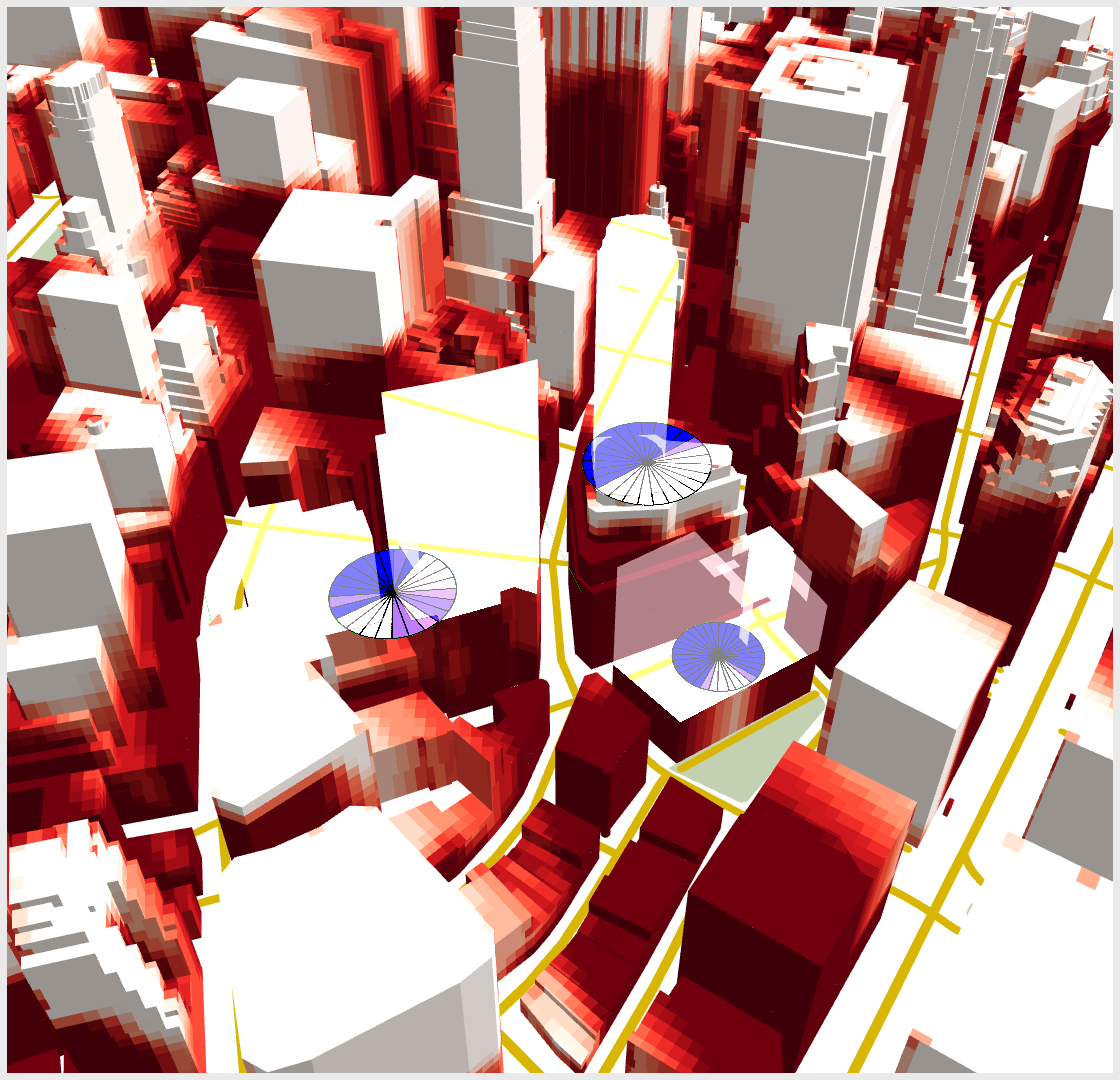
Final result
{
  "components": [
    {
      "map": {
        "camera": {
          "position": [
            -8239611,
            4941390.5,
            2.100369140625
          ],
          "direction": {
            "right": [
              553.601318359375,
              -2370.810546875,
              2100.369140625
            ],
            "lookAt": [
              563.9249267578125,
              -1633.5897216796875,
              1424.7962646484375
            ],
            "up": [
              0.009459096007049084,
              0.6755067110061646,
              0.7372931241989136
            ]
          }
        },
        "knots": [
          "purewater",
          "pureroads",
          "buildings"
        ],
        "interactions": [
          "NONE",
          "NONE",
          "NONE"
        ]
      },
      "plots": [
        {
          "plot": {
            "$schema": "https://vega.github.io/schema/vega-lite/v5.json",
            "background": "rgb(0,255,0)",
            "mark": {
              "type": "arc",
              "stroke": "black",
              "strokeWidth": 5
            },
            "encoding": {
                "theta": {
                "field": "bin",
                "type": "nominal",
                "legend": null
              },
              "color": {
                "field": "buildings_abstract",
                "type": "quantitative",
                "aggregate": "mean",
                "legend": null,
                "scale": {
                  "scheme": [
                    "white",
                    "white",
                    "blue"
                  ]
                }
              }
            }
          },
          "knots": [
            "buildings"
          ],
          "arrangement": "FOOT_EMBEDDED",
          "args": {
            "bins": 32
          }
        }
      ],
      "knots": [
        {
          "id": "purewater",
          "integration_scheme": [
            {
              "out": {
                "name": "water",
                "level": "OBJECTS"
              }
            }
          ]
        },
        {
          "id": "pureroads",
          "integration_scheme": [
            {
              "out": {
                "name": "roads",
                "level": "OBJECTS"
              }
            }
          ]
        },
        {
          "id": "buildings",
          "integration_scheme": [
            {
              "spatial_relation": "NEAREST",
              "out": {
                "name": "buildings",
                "level": "COORDINATES3D"
              },
              "in": {
                "name": "shadow",
                "level": "COORDINATES3D"
              },
              "operation": "NONE",
              "abstract": true
            }
          ]
        }
      ],
      "position": {
        "width": [
          6,
          12
        ],
        "height": [
          1,
          5
        ]
      }
    },
    {
      "type": "GRAMMAR",
      "position": {
        "width": [
          1,
          5
        ],
        "height": [
          3,
          4
        ]
      }
    },
    {
      "type": "TOGGLE_KNOT",
      "map_id": 0,
      "position":{
        "width": [
          1,
          5
        ],
        "height": [
          1,
          2
        ]
      }
    }
  ],
  "arrangement": "LINKED",
  "grid": {
    "width": 12,
    "height": 4
  }
}