What-if Scenario
You can download the data here to quickly run this example locally. Please refer to the GitHub repository for instructions on how to start the Urban Toolkit on your machine.
Step 0 – Open web editor
You are going to encounter an initial blank setup (right image) when opening the web editor for the first time. On the left side, we have the grammar editor describing basic structures of the grammar such as a map component, grid configuration, grammar component, and toggle knots component. The right side, on the other hand, is the result of this basic specification.
– Map component: defines position and direction of the camera, how to integrate and render data (“knots”), interactions, plots, and the position of the map on the screen of the application (according to a grid).
– Grid configuration: defines how the screen will be divided. “width” for the number of columns. “height” for the number of rows.
– Grammar component: defines the position of the grammar editor.
– Toggle knots component: defines a widget that supports the toggle of knots.

Step 1 – Adding background layer (water)
To start rendering our scene we are going to add a basic water layer containing the ocean.
The water layer as well as all other layers were previously generated using the the Jupyter API. In order to load it we have to add:
– A knot that contains a pure physical layer (no thematic data). It specifies that we want to output the water layer on the objects level (we want the shapes not coordinates).
– A reference to that knot on the map component.
– The type of interaction we want to have with the knot (none in this case).
* All required changes are highlighted in red. Sections of the code where nothing changed have “…”. After adding them hit Apply Grammar.
{
  "components": [
    {
      "map": {
        "camera": {...},
          "knots": [
            "purewater"
          ],
          "interactions": [
            "NONE"
          ]
      },
      "plots": [],
      "knots": [
        {
          "id": "purewater",
          "integration_scheme": [
            {
              "out": {
                "name": "water",
                "level": "OBJECTS"
              }
            }
          ]
        }
      ],
      "position": {...}
    },
    {
      "type": "GRAMMAR",
      "position": {...}
    },
    {
      "type": "TOGGLE_KNOT",
      "map_id": 0,
      "position":{...}
    }
  ],
  "arrangement": "LINKED",
  "grid": {...}
}
Step 2 – Adding other background layers (parks and roads)
Just as we did in Step 1, we are going to define and render pure “knots” for parks and roads as well. The steps are analogous.
* All required changes are highlighted in red. Sections of the code where nothing changed have “…”. After adding them hit Apply Grammar.
{
  "components": [
    {
      "map": {
        "camera": {...},
          "knots": [
            ...
            "pureparks",
            "pureroads"
          ],
          "interactions": [
            ...
            "NONE",
            "NONE"
          ]
      },
      "plots": [],
      "knots": [
        ...
        {
          "id": "pureparks",
          "integration_scheme": [
            {
              "out": {
                "name": "parks",
                "level": "OBJECTS"
              }
            }
          ]
        },
        {
          "id": "pureroads",
          "integration_scheme": [
            {
              "out": {
                "name": "roads",
                "level": "OBJECTS"
              }
            }
          ]
        }
      ],
      "position": {...}
    },
    {
      "type": "GRAMMAR",
      "position": {...}
    },
    {
      "type": "TOGGLE_KNOT",
      "map_id": 0,
      "position":{...}
    }
  ],
  "arrangement": "LINKED",
  "grid": {...}
}
Step 3 – Adding buildings and surfaces
Adding a 3D layer with the buildings is as simple as adding water, parks, and roads. The data for this Step was retrieved from OpenStreetMap (OSM) and parsed by the JupyterAPI. In this example, since we want to compare the shadow impact of a few buildings, we are going to load buildings and buildings_m where the last one does not have the buildings we want to analyze.
Besides the buildings, we are also going to render two heatmap surfaces (without thematic data for now) that will contain the shadow simulation results for the two scenarios.
* All required changes are highlighted in red. Sections of the code where nothing changed have “…”. After adding them hit Apply Grammar.
{
  "components": [
    {
      "map": {
        "camera": {...},
          "knots": [
            ...
            "surface",
            "surface_m",
            "buildings",
            "buildings_m"
          ],
          "interactions": [
            ...
            "NONE",
            "NONE",
            "BRUSHING",
            "BRUSHING"
          ]
      },
      "plots": [],
      "knots": [
        ...
        {
          "id": "surface",
          "integration_scheme": [
            {
              "out": {
                "name": "surface",
                "level": "OBJECTS"
              }
            }
          ]
        },
        {
          "id": "surface_m",
          "integration_scheme": [
            {
              "out": {
                "name": "surface",
                "level": "OBJECTS"
              }
            }
          ]
        },
        {
          "id": "buildings",
          "integration_scheme": [
            {
              "out": {
                "name": "buildings",
                "level": "OBJECTS"
              }
            }
          ]
        },
        {
          "id": "buildings_m",
          "integration_scheme": [
            {
              "out": {
                "name": "buildings_m",
                "level": "OBJECTS"
              }
            }
          ]
        }
      ],
      "position": {...}
    },
    {
      "type": "GRAMMAR",
      "position": {...}
    },
    {
      "type": "TOGGLE_KNOT",
      "map_id": 0,
      "position":{...}
    }
  ],
  "arrangement": "LINKED",
  "grid": {...}
}
Step 4 – Adding shadow data on top of the buildings and surfaces
In all previous Steps we added pure “knots” that did not have thematic data. In this example, we are going to add the results of two runs of shadow simulations made on 12/26/2015 accumulated between 15:00 and 17:01 on top of the buildings and surface. One of the runs calculated the ray tracing including all the buildings and the other one excluded a few buildings. To do that some small changes to the previous knot definitions are necessary:
– New input layers for the thematic data.
– Adding spatial_relation to define the spatial join that will link physical and thematic layers.
– Adding operation to indicate how to aggregate the result of the spatial joins (none, because we have a 1:1 relation).
– An abstract flag to indicate that thematic data is being joined with the physical.
– The geometry level of all layers is now “coordinates”. Since we want to have heatmaps (on the buildings and on the surface) we need a different scalar value for each coordinate of the meshes.
* All required changes are highlighted in red. All tweaks are highlighted in blue. Sections of the code where nothing changed have “…”. After adding them hit Apply Grammar.
{
  "components": [
    {
      "map": {
        "camera": {...},
          "knots": [
            ...
          ],
          "interactions": [
            ...
          ]
      },
      "plots": [],
      "knots": [
        ...
        {
          "id": "surface",
          "integration_scheme": [
            {
              "spatial_relation": "NEAREST",
              "out": {
                "name": "surface",
                "level": "COORDINATES3D"
              },
              "in": {
                "name": "shadow_surface",
                "level": "COORDINATES3D"
              },
              "operation": "NONE",
              "abstract": true
            }
          ]
        },
        {
          "id": "surface_m",
          "integration_scheme": [
            {
              "spatial_relation": "NEAREST",
              "out": {
                "name": "surface_m",
                "level": "COORDINATES3D"
              },
              "in": {
                "name": "shadow_surface_m",
                "level": "COORDINATES3D"
              },
              "operation": "NONE",
              "abstract": true
            }
          ]
        },
        {
          "id": "buildings",
          "integration_scheme": [
            {
              "spatial_relation": "NEAREST",
              "out": {
                "name": "buildings",
                "level": "COORDINATES3D"
              },
              "in": {
                "name": "shadow",
                "level": "COORDINATES3D"
              },
              "operation": "NONE",
              "abstract": true
            }
          ]
        },
        {
          "id": "buildings_m",
          "integration_scheme": [
            {
              "spatial_relation": "NEAREST",
              "out": {
                "name": "buildings_m",
                "level": "COORDINATES3D"
              },
              "in": {
                "name": "shadow_m",
                "level": "COORDINATES3D"
              },
              "operation": "NONE",
              "abstract": true
            }
          ]
        }
      ],
      "position": {...}
    },
    {
      "type": "GRAMMAR",
      "position": {...}
    },
    {
      "type": "TOGGLE_KNOT",
      "map_id": 0,
      "position":{...}
    }
  ],
  "arrangement": "LINKED",
  "grid": {...}
}
Step 5 – Operating knots
UTK allows us to define operations between knots. We can use that feature to highlight the differences between the two simulation scenarios we loaded in Step 3. The operation of two knots is defined by a third knot that stores the result of the operation. In order to do that some changes to the code are necessary:
– Knots that store the result of operations need to have two special fields: knotOp (indicates that a knot operation is happening) and op (an arithmetic operation that will be applied on the knots). It is important to notice that in this case in and out point to knots instead of layers.
– Adding colorMap field to use d3 blue color scale to highlight differences.
– Remove the references to buildings and surfaces knots on the map, since it is already being rendered as a result of the knot operations.
– Change the out layer of the “buildings” knot to “buildings_m” instead of “buildings”. We need to make this change because the operated knots need to have the same number of elements.
* All required changes are highlighted in red. All tweaks are highlighted in blue. All removed code is highlighted with a strikethrough. Sections of the code where nothing changed have “…”. After adding them hit Apply Grammar.
{
  "components": [
    {
      "map": {
        "camera": {...},
          "knots": [
            ...
            "whatIfSurface",
            "whatIfBuildings"
            "surface",
            "surface_m",
            "buildings",
            "buildings_m"
          ],
          "interactions": [
            ...
            "NONE",
            "NONE"
          ]
      },
      "plots": [],
      "knots": [
        ...
        {
          "id": "buildings",
          "integration_scheme": [
            {
              "spatial_relation": "NEAREST",
              "out": {
                "name": "buildings_m",
                "level": "COORDINATES3D"
              },
              "in": {
                "name": "shadow",
                "level": "COORDINATES3D"
              },
              "operation": "NONE",
              "abstract": true
            }
          ]
        },
        {
          "id": "whatIfSurface",
          "knotOp": true,
          "colorMap": "interpolateBlues",
          "integration_scheme": [
            {
              "out": {
                "name": "surface_m",
                "level": "COORDINATES3D"
              },
              "in": {
                "name": "surface",
                "level": "COORDINATES3D"
              },
              "op": "surface - surface_m",
              "operation": "NONE"
            }
          ]
        },
        {
          "id": "whatIfBuildings",
          "knotOp": true,
          "colorMap": "interpolateBlues",
          "integration_scheme": [
            {
              "out": {
                "name": "buildings_m",
                "level": "COORDINATES3D"
              },
              "in": {
                "name": "buildings",
                "level": "COORDINATES3D"
              },
              "op": "buildings - buildings_m",
              "operation": "NONE"
            }
          ]
        }
      ],
      "position": {...}
    },
    {
      "type": "GRAMMAR",
      "position": {...}
    },
    {
      "type": "TOGGLE_KNOT",
      "map_id": 0,
      "position":{...}
    }
  ],
  "arrangement": "LINKED",
  "grid": {...}
}
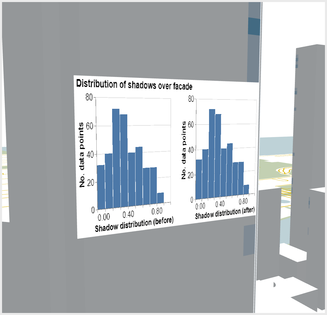
Step 6 – Adding embedded distribution plot
To enhance the analytical capabilities of our system, UTK gives support to the use of customized Vega-Lite plots. To help us compare the difference between the two shadow scenarios we are going to create a distribution plot that will be embedded on the surface of the buildings. Notice that we are using plain vega with the difference that it is possible to use keywords to make references to the knots inside the specification. Each plot has four fields: plot (vega specification), knots (id of the knots to be used on the plot), arrangement (where the plot will be located), and interaction. In our case, the arrangement is “SUR_EMBEDDED” as opposed to “FOOT_EMBEDDED” or “LINKED” because we want the plots to be on the surface of the building.
To access knot data inside the vega specification one can use the structure “knotId_keyword”. The keyword can be “abstract” (the thematic data), “index” (the index of the element on the knot), and “highlight” a boolean indicating if the element of the knot is highlighted. In Step 3 we configured our “buildings” and “buildings_m” knots to have a “BRUSHING” interaction which means that we can choose where to embed the visualization by using “alt + left-click mouse + drag” and “enter” to confirm and the “buildings_highlight” variable inside the vega specification will be true for that set of points. To deselect a section you can use “right-click mouse” and remove all plots with “r”.
* Allow some seconds of delay when brushing and applying the plot
{
  "components": [
    {
      "map": {
        "camera": {...},
          "knots": [
            ...
          ],
          "interactions": [
            ...
          ]
      },
      "plots": [
        {
          "plot": {
            "title": {
              "text": "Distribution of shadows over facade",
              "fontSize": 18
            },
            "hconcat": [
              {
                "mark": "bar",
                "encoding": {
                  "x": {
                    "bin": {"extent": [0,1]},
                    "field": "buildings_abstract",
                    "axis": {
                      "title": "Shadow distribution (before)",
                      "titleFontSize": 16,
                      "labelFontSize": 16
                    }
                  },
                  "y": {
                    "aggregate": "count",
                    "axis": {
                      "title": "No. data points",
                      "titleFontSize": 16,
                      "labelFontSize": 16
                  }
                }
              }
            },
            {
              "mark": "bar",
              "encoding": {
                "x": {
                  "bin": {"extent": [0,1]},
                  "field": "buildings_m_abstract",
                  "axis": {
                    "title": "Shadow distribution (after)",
                    "titleFontSize": 16,
                    "labelFontSize": 16
                  }
                },
                "y": {
                  "aggregate": "count",
                  "axis": {
                    "title": "No. data points",
                    "titleFontSize": 16,
                    "labelFontSize": 16
                  }
                }
              }
            }
          ]
        },
          "knots": [
            "buildings",
            "buildings_m"
          ],
          "arrangement": "SUR_EMBEDDED"
        }
      ],
      "knots": [
        ...
      ],
      "position": {...}
    },
    {
      "type": "GRAMMAR",
      "position": {...}
    },
    {
      "type": "TOGGLE_KNOT",
      "map_id": 0,
      "position":{...}
    }
  ],
  "arrangement": "LINKED",
  "grid": {...}
}
Final result
{
  "components": [
    {
      "map": {
        "camera": {
          "position": [
            -9754472.41870091,
            5115000.8427740205,
            1
          ],
          "direction": {
            "right": [
              0,
              0,
              3000
            ],
            "lookAt": [
              0,
              0,
              0
            ],
            "up": [
              0,
              1,
              0
            ]
          }
        },
        "knots": [
          "purewater",
          "pureparks",
          "pureroads",
          "whatIfSurface",
          "whatIfBuildings"
        ],
        "interactions": [
          "NONE",
          "NONE",
          "NONE",
          "NONE",
          "NONE"
        ]
      },
      "plots": [
        {
          "plot": {
            "title": {
              "text": "Distribution of shadows over facade",
              "fontSize": 18
            },
            "hconcat": [
              {
                "mark": "bar",
                "encoding": {
                  "x": {
                    "bin": {"extent": [0,1]},
                    "field": "buildings_abstract",
                    "axis": {
                      "title": "Shadow distribution (before)",
                      "titleFontSize": 16,
                      "labelFontSize": 16
                    }
                  },
                  "y": {
                    "aggregate": "count",
                    "axis": {
                      "title": "No. data points",
                      "titleFontSize": 16,
                      "labelFontSize": 16
                  }
                }
              }
            },
            {
              "mark": "bar",
              "encoding": {
                "x": {
                  "bin": {"extent": [0,1]},
                  "field": "buildings_m_abstract",
                  "axis": {
                    "title": "Shadow distribution (after)",
                    "titleFontSize": 16,
                    "labelFontSize": 16
                  }
                },
                "y": {
                  "aggregate": "count",
                  "axis": {
                    "title": "No. data points",
                    "titleFontSize": 16,
                    "labelFontSize": 16
                  }
                }
              }
            }
          ]
        },
          "knots": [
            "buildings",
            "buildings_m"
          ],
          "arrangement": "SUR_EMBEDDED"
        }
      ],
      "knots": [
        {
          "id": "purewater",
          "integration_scheme": [
            {
              "out": {
                "name": "water",
                "level": "OBJECTS"
              }
            }
          ]
        },
        {
          "id": "pureparks",
          "integration_scheme": [
            {
              "out": {
                "name": "parks",
                "level": "OBJECTS"
              }
            }
          ]
        },
        {
          "id": "pureroads",
          "integration_scheme": [
            {
              "out": {
                "name": "roads",
                "level": "OBJECTS"
              }
            }
          ]
        },
        {
          "id": "surface",
          "integration_scheme": [
            {
              "spatial_relation": "NEAREST",
              "out": {
                "name": "surface",
                "level": "COORDINATES3D"
              },
              "in": {
                "name": "shadow_surface",
                "level": "COORDINATES3D"
              },
              "abstract": true,
              "operation": "NONE"
            }
          ]
        },
        {
          "id": "surface_m",
          "integration_scheme": [
            {
              "spatial_relation": "NEAREST",
              "out": {
                "name": "surface",
                "level": "COORDINATES3D"
              },
              "in": {
                "name": "shadow_surface_m",
                "level": "COORDINATES3D"
              },
              "abstract": true,
              "operation": "NONE"
            }
          ]
        },
        {
          "id": "buildings",
          "integration_scheme": [
            {
              "spatial_relation": "NEAREST",
              "out": {
                "name": "buildings_m",
                "level": "COORDINATES3D"
              },
              "in": {
                "name": "shadow",
                "level": "COORDINATES3D"
              },
              "abstract": true,
              "operation": "NONE"
            }
          ]
        },
        {
          "id": "buildings_m",
          "integration_scheme": [
            {
              "spatial_relation": "NEAREST",
              "out": {
                "name": "buildings_m",
                "level": "COORDINATES3D"
              },
              "in": {
                "name": "shadow_m",
                "level": "COORDINATES3D"
              },
              "abstract": true,
              "operation": "NONE"
            }
          ]
        },
        {
          "id": "whatIfSurface",
          "knotOp": true,
          "colorMap": "interpolateBlues",
          "integration_scheme": [
            {
              "out": {
                "name": "surface_m",
                "level": "COORDINATES3D"
              },
              "in": {
                "name": "surface",
                "level": "COORDINATES3D"
              },
              "op": "surface - surface_m",
              "operation": "NONE"
            }
          ]
        },
        {
          "id": "whatIfBuildings",
          "knotOp": true,
          "colorMap": "interpolateBlues",
          "integration_scheme": [
            {
              "out": {
                "name": "buildings_m",
                "level": "COORDINATES3D"
              },
              "in": {
                "name": "buildings",
                "level": "COORDINATES3D"
              },
              "op": "buildings - buildings_m",
              "operation": "NONE"
            }
          ]
        }
      ],
      "position": {
        "width": [
          6,
          12
        ],
        "height": [
          1,
          5
        ]
      }
    },
    {
      "type": "GRAMMAR",
      "position": {
        "width": [
          1,
          5
        ],
        "height": [
          3,
          5
        ]
      }
    },
    {
      "type": "TOGGLE_KNOT",
      "map_id": 0,
      "position":{
        "width": [
          1,
          5
        ],
        "height": [
          1,
          2
        ]
      }
    }
  ],
  "arrangement": "LINKED",
  "grid":{
    "width": 12,
    "height": 5
  }
}