Getting Started
Tutorials
For a hands-on experience with the Urban Toolkit please refer to the tutorials page. A web editor is provided and no previous experience is needed.
Installation
If you want to run the Urban Toolkit locally, please refer to our GitHub page.
By default, UTK will be available on localhost:5001.
The Urban Toolkit architecture
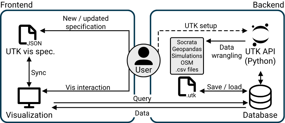
Frontend
Urban Toolkit is the core of the project and is responsible for interpreting the grammar, allowing interactions with the rendered visual analytics system, and providing a general interface of access to the grammar. The Urban Toolkit depends on available data to be used since it assumes that data is already available in the correct format. For the tutorials previously mentioned the web editor is the Urban Toolkit. In the context of this guide, UTK is available in localhost:5001.
Python API
The Jupyter API is a service based on Jupyter Notebook that supports the download and transformation of data in order to provide an adequate format for UTK. For example, it is possible to load several layers from OpenStreetMap (OSM) or transform a CSV file into a thematic layer. For the tutorials previously mentioned the data is already prepared so there is no need to use the API.
Map interactions
- left click + drag to move the camera
- mouse wheel to zoom in and zoom out
- shift + left-click to rotate the camera
- t to select a building/embed plots
- alt + mouse wheel to change the height of an embedded plot
- r to reset embedded plots
- shift + left-click + drag to brush on the surface of buildings
- enter to apply brush
- right-click to reset brushing and selections
Configuration
UTK leverages several spatial packages, such as Geopandas, OSMnx, Osmium, Shapely. To facilite the installation of UTK, we have made it available through pip, only requiring the following commands in a terminal / command prompt:
pip install utkUTK requires Python 3.9 or a newer version. If you are having problems installing UTK in Mac OSX because of Osmium, make sure you have CMake installed as well (e.g., through conda or Homebrew). A detailed description of UTK’s capabilities can be found in our paper, but generally speaking UTK is divided into two components: a backend component, accessible through UTK’s Python library, and a frontend component, accessible through a web interface.
Hands-on
To exemplify how Urban Toolkit and the Python API can work together to build a visual analytics system from scratch, a step-by-step introductory example will be provided. The goal of this example is to load water, parks, and building layers of Downtown NYC from OpenStreetMap (OSM) using the Python API and render that data into a map using the Urban Toolkit.
Step 0 – Setup
The following setup steps are required:
– A folder data/my_first_vis should be created at the root of the project.
– Start the services using utk start.
Step 1 – Downloading layers from OSM
For this Step, we need to use the Python API. Create a Jupyter notebook (using Jupyter or JupyterLab):

Create a coding block inside the Jupyter Notebook of the following content:
import utk
This line of code imports the python API that will be used to load the OSM layers.
Create another block of code and add:
uc = utk.OSM.load([40.699768, -74.019904, 40.71135, -74.004712], layers=['water', 'surface', 'parks', 'roads', 'buildings'])
uc.save('./data/my_first_vis', includeGrammar=False)
The first line uses the OSM submodule of the API to load all the layers that we want. We are specifying the location of the data we want to load through a bounding box with a format [minLat, minLong, maxLat, maxLong]. In this case, that bounding box encompasses a region of Downtown NYC.
The second line indicates that we want to save the content of what was loaded inside the data folder we created previously. As one can notice we set the includeGrammar to be false, which means that the grammar file will not be automatically generated. This flag was deactivated so we can build the grammar from scratch, but letting it generate the grammar is useful in most cases.
After including all those lines of code you can run the Jupyter Notebook and after a few seconds, the files will be produced.
Step 2 – Simulating shadows
To facilitate the incorporation of shadow (since a compatible GPU is not available in all computers) you can download the shadow simulation for this specific region of NYC here.

Step 3 – UTK setup
Now that we have the data files, we can start using the Urban Toolkit to render the data. But before we can do that, we have to create a grammar.json file inside data/my_first_vis, since that was not created in Step 1.
To start the UTK server, on the command line, type utk start. For the initial setup, we are going to include the following code inside grammar.json and go to localhost:3000:
{
  "components": [
    {
      "map": {
        "camera": {
          "position": [
            -8239611,
            4941390.5,
            2.100369140625
          ],
          "direction": {
            "right": [
              553.601318359375,
              -2370.810546875,
              2100.369140625
            ],
            "lookAt": [
              563.9249267578125,
              -1633.5897216796875,
              1424.7962646484375
            ],
            "up": [
              0.009459096007049084,
              0.6755067110061646,
              0.7372931241989136
            ]
          }
        },
        "knots": [],
        "interactions": []
      },
      "plots": [],
      "knots": [],
      "widgets": [
        {
          "type": "TOGGLE_KNOT"
        }
      ],
      "position": {
        "width": [
          6,
          12
        ],
        "height": [
          1,
          4
        ]
      }
    }
  ],
  "arrangement": "LINKED",
  "grid": {
    "width": 12,
    "height": 4
  },
  "grammar_position": {
    "width": [
1,
5
],
    "height": [
1,
4
]
  }
}
The image included in this Step is the initial setup you are going to encounter when opening UTK for the first time. On the left side, we have the grammar editor describing basic structures of the grammar such as a map component, grid configuration, grammar component, and toggle knots component. The right side, on the other hand, is the result of this basic specification, which is empty for now since we have not added the data we generated yet.
Map component: defines position and direction of the camera, how to integrate and render data (“knots”), interactions, plots, and the position of the map on the screen of the application (according to a grid).
Grid configuration: defines how the screen will be divided. “width” for the number of columns. “height” for the number of rows.
Grammar component: defines the position of the grammar editor.
Toggle knots component: defines a widget that supports the toggle of knots.
Step 4 – Adding background layer (water)
To start rendering our scene we, are going to add the water layer we loaded in Step 1.
The water layer as well as all other layers were previously generated using the the Jupyter API. In order to load it we have to add:
– A knot that contains a pure physical layer (no thematic data). It specifies that we want to output the water layer on the objects level (we want the shapes not coordinates).
– A reference to that knot on the map component.
– The type of interaction we want to have with the knot (none in this case).
* All required changes are highlighted in red. Sections of the code where nothing changed have “…”. After adding them hit Apply Grammar.
{
  "components": [
    {
      "map": {
        "camera": {...},
          "knots": [
            "purewater"
          ],
          "interactions": [
            "NONE"
          ]
      },
      "plots": [],
      "knots": [
        {
          "id": "purewater",
          "integration_scheme": [
            {
              "out": {
                "name": "water",
                "level": "OBJECTS"
              }
            }
          ]
        }
      ],
      "widgets": [...
],
      "position": {...}
    }
  ],
  "arrangement": "LINKED",
  "grid": {...},
  "grammar_position": {...}
}
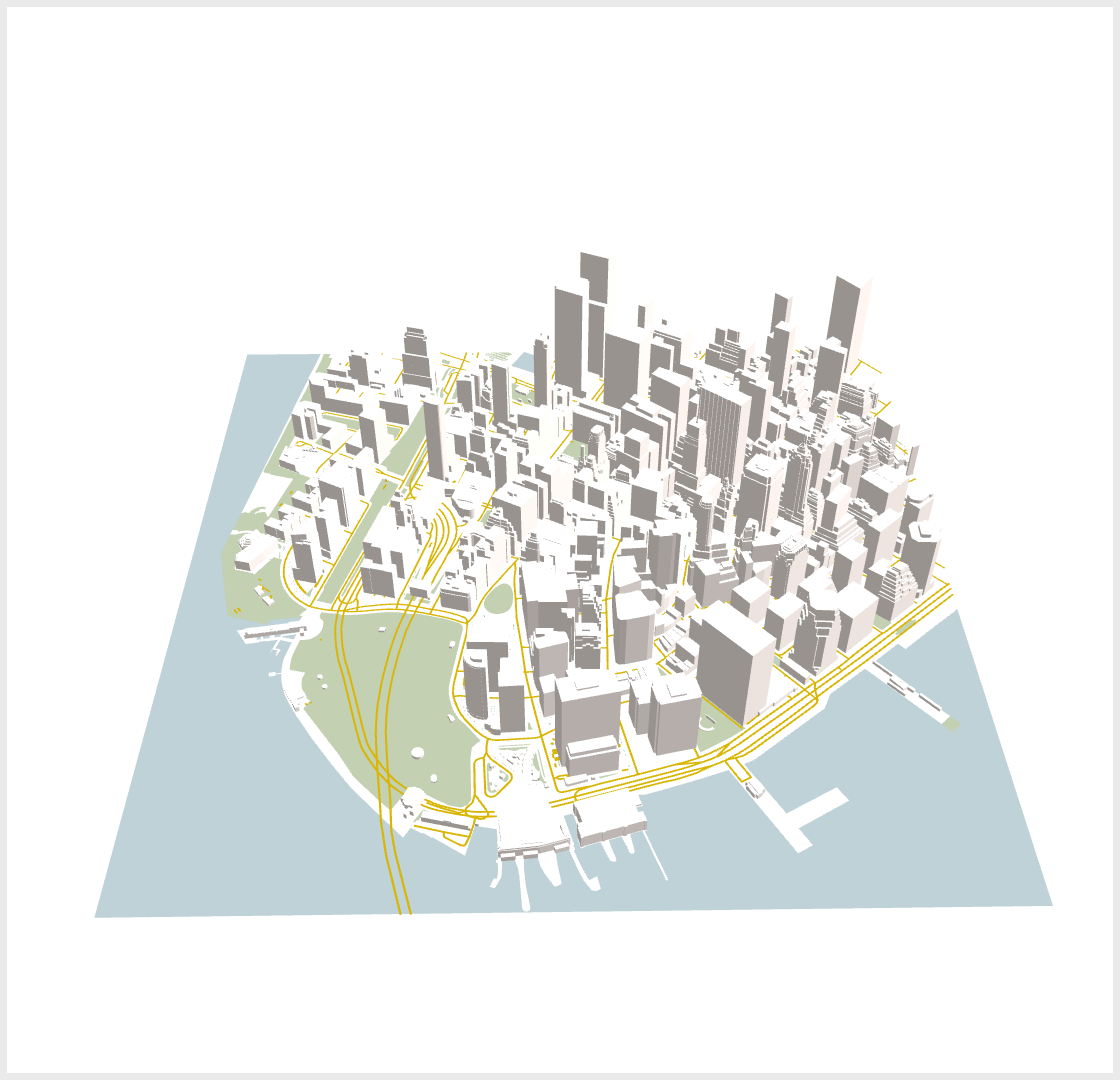
Step 5 – Adding all the other layers
Since this is a simple example where all the layers only have physical data and not thematic data, the way the other layers are loaded is very similar.
* All required changes are highlighted in red. Sections of the code where nothing changed have “…”. After adding them hit Apply Grammar.
{
  "components": [
    {
      "map": {
        "camera": {...},
          "knots": [
            ...
            "pureparks",
            "pureroads",
            "buildings"
          ],
          "interactions": [
            ...
            "NONE",
            "NONE",
            "NONE"
          ]
      },
      "plots": [],
      "knots": [
        ...
        {
          "id": "pureparks",
          "integration_scheme": [
            {
              "out": {
                "name": "parks",
                "level": "OBJECTS"
              }
            }
          ]
        },
        {
          "id": "pureroads",
          "integration_scheme": [
            {
              "out": {
                "name": "roads",
                "level": "OBJECTS"
              }
            }
          ]
        },
        {
          "id": "buildings",
          "integration_scheme": [
            {
              "out": {
                "name": "buildings",
                "level": "OBJECTS"
              }
            }
          ]
        }
      ],
      "widgets": [...]
      "position": {...}
    }
  ],
  "arrangement": "LINKED",
  "grid": {...},
  "grammar_position": {...}
}
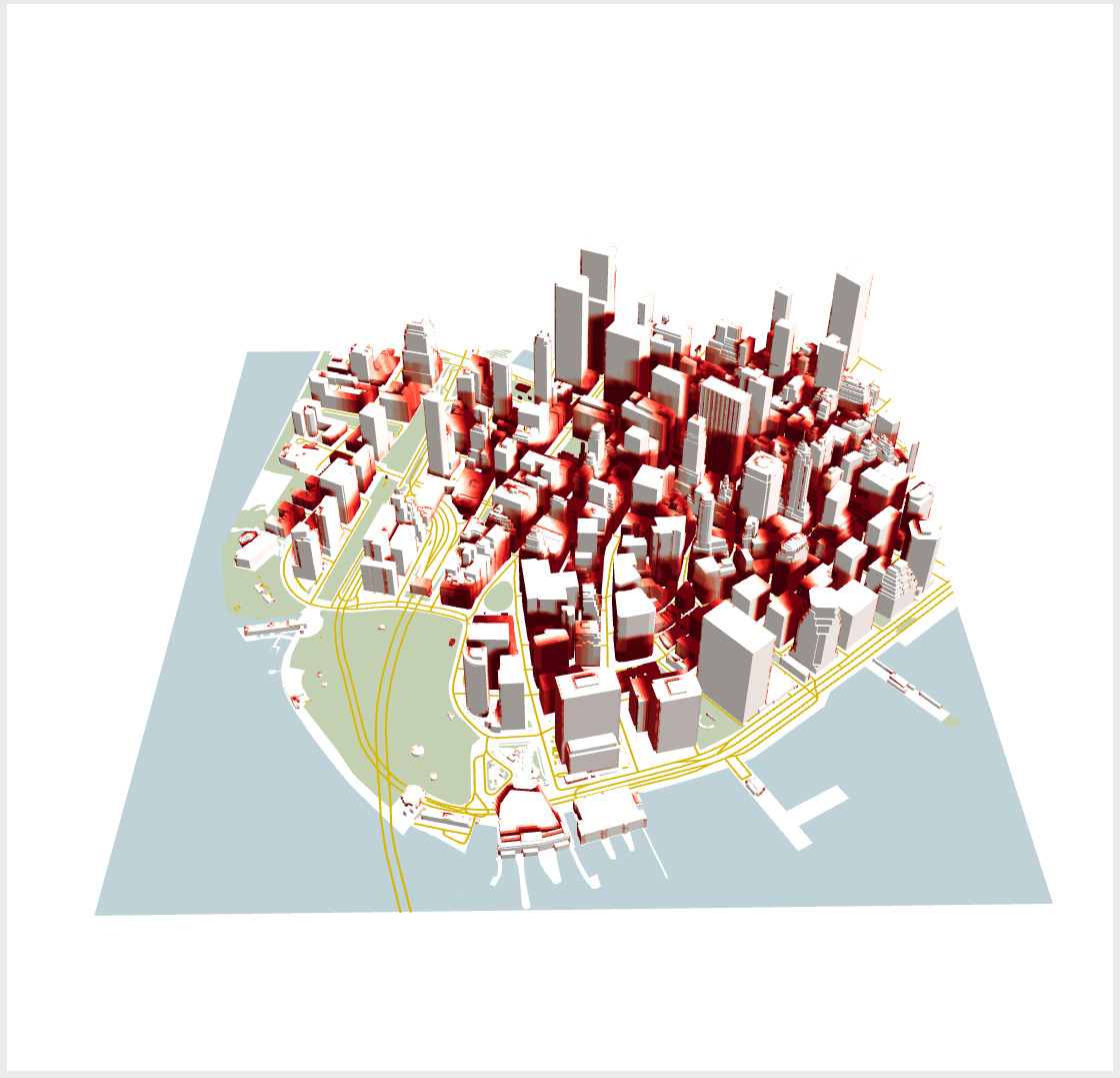
Step 6 – Attaching Shadows
In all previous Steps we added pure “knots” that did not have thematic data. In this example, we are going to add the results of the shadow simulation on top of the buildings. That requires some small changes to the knot definition:
– A new input layer for the thematic data.
– A spatial_relation to define the spatial join that will link physical and thematic layers.
– An operation to indicate how to aggregate the result of the spatial join (none, because we have a 1:1 relation).
– An abstract flag to indicate that thematic data is being joined with the physical.
– The geometry level of both layers is now “coordinates”. Since we want to have a heatmap we need a different scalar value for each coordinate of the buildings.
* All required changes are highlighted in red. All tweaks are highlighted in blue. Sections of the code where nothing changed have “…”. After adding them hit Apply Grammar.
{
  "components": [
    {
      "map": {
        "camera": {...},
          "knots": [
            ...
          ],
          "interactions": [
            ...
          ]
      },
      "plots": [],
      "knots": [
        ...
        {
          "id": "buildings",
          "integration_scheme": [
            {
              "spatial_relation": "NEAREST",
              "out": {
                "name": "buildings",
                "level": "COORDINATES3D"
              },
              "in": {
                "name": "shadow",
                "level": "COORDINATES3D"
              },
              "operation": "NONE",
              "abstract": true
            }
          ]
        }
      ],
      "widgets": [...]
      "position": {...}
    }
  ],
  "arrangement": "LINKED",
  "grid": {...},
  "grammar_position": {...}
}
Final Result
{
  "components": [
    {
      "map": {
        "camera": {
          "position": [
            -8239611,
            4941390.5,
            2.100369140625
          ],
          "direction": {
            "right": [
              553.601318359375,
              -2370.810546875,
              2100.369140625
            ],
            "lookAt": [
              563.9249267578125,
              -1633.5897216796875,
              1424.7962646484375
            ],
            "up": [
              0.009459096007049084,
              0.6755067110061646,
              0.7372931241989136
            ]
          }
        },
        "knots": [
            "purewater",
            "pureparks",
            "pureroads",
            "buildings"
        ],
        "interactions": [
          "NONE",
          "NONE",
          "NONE",
          "NONE"
        ]
      },
      "plots": [],
      "knots": [
        {
          "id": "purewater",
          "integration_scheme": [
            {
              "out": {
                "name": "water",
                "level": "OBJECTS"
              }
            }
          ]
        },
        {
          "id": "pureparks",
          "integration_scheme": [
            {
              "out": {
                "name": "parks",
                "level": "OBJECTS"
              }
            }
          ]
        },
        {
          "id": "pureroads",
          "integration_scheme": [
            {
              "out": {
                "name": "roads",
                "level": "OBJECTS"
              }
            }
          ]
        },
        {
          "id": "buildings",
          "integration_scheme": [
            {
              "spatial_relation": "NEAREST",
              "out": {
                "name": "buildings",
                "level": "COORDINATES3D"
              },
              "in": {
                "name": "shadow",
                "level": "COORDINATES3D"
              },
              "operation": "NONE",
              "abstract": true
            }
          ]
        }
      ],
      "widgets": [...]
      "position": {
        "width": [
          6,
          12
        ],
        "height": [
          1,
          4
        ]
      }
    }
  ],
  "arrangement": "LINKED",
  "grid": {
    "width": 12,
    "height": 4
  },
  "grammar_position": {
    "width": [
1,
5
],
    "height": [
1,
4
]
  }
}
In a few steps, we went from zero to having a customized visual analytics system to visualize data downloaded from OpenStreetMap. However, the capabilities of UTK do not stop here and we encourage you to refer to the tutorials page if you want a more in-depth guide for the tool.
Full documentation
The content of this page is a gentle introduction to the Urban Toolkit and its capabilities. The full documentation for the Grammar can be found here and for the Jupyter API here.